2. Front End Module

2.1. Camera Projection model

In SLAM problem, the objective is to estimate the motion of the sensor in 3D space with a set of measurement data provided by monocular or stereo camera. To further perform the pose recovery, the pose to be estimated has to be represented by a set of parameters, as well as the observed landmarks.

Firstly, in the report we use homogeneous points with unit-length \(4\times1\) columns to represent Euclidean points, which are the observed landmarks, namely feature points: \(\mathbf{p}_i=\left[x_i,y_i,z_i,1\right]^\intercal\).

Secondly, the parametrization of sensor state \(\mathbf{T}(k) \in{\mathbb{R}^{4\times4}}\) is described by a \(4\times4\) transformation matrix which represents the element of the group SE(3):

(2.1)\[\begin{split}\begin{equation} \mathbf{T}(k) = \begin{bmatrix} \mathbf{R}_k & \mathbf{t}_k \\ \mathbf{0} & 1 \end{bmatrix} \quad \text{with} \quad \mathbf{R}\in{\mathrm{SO(3)}}\quad \text{and}\quad \mathbf{t}\in{\mathbb{R}^3} \end{equation}\end{split}\]

Usually we use rigid body transformation matrix \(\mathbf{T}_{c}^w(k)\) to map the camera coordinate frame at time \(k\) into the world frame \(w\), such that a point \(\mathbf{p}_k\in{\mathbb{R}^3}\) in the camera frame is transferred into the world coordinate frame: \(\mathbf{p}_k^w=\mathbf{T}_{c}^w(k)\mathbf{p}_k^c\).

Most of the early work used Euler angles and rotation matrices as the parametrization for rotations. However, Euler angles in Euclidean spaces is not properly invariant under rigid transformations, not to mention the singularity. What’s more, the rotation matrix is self-constrained (orthogonal and determinant equals to 1), so when we optimize it, additional constraints makes the optimization extremely difficult. Therefore the better way is to introduce the transformation between Lie-group and Lie-algebra which turns the pose estimation problem into unconstrained optimization problem and deal with state variables that span over non-Euclidean space. Therefore we use Lie-algebra to represent the pose using the corresponding element \(\mathbf{\xi}\in{\mathfrak{se}(3)}\) during the optimization process. The elements are mapped to \(\mathrm{SE(3)}\) with exponential map \(\mathfrak{se}(3)\to \mathrm{SE(3)}\):

(2.2)\[\begin{equation} \text{exp}(\mathbf{\xi}_k^{\wedge})=\mathbf{T}(k) \end{equation}\]

During optimization, derivative is the key information. So the advantage of using Lie-algebra to represent pose is that in the tangent space on the manifold \(\mathrm{SO(3)}\), we can use the perturbation model to easily approximate the derivative of the incremental rotation 4.

On the other hand, let’s review the process of projection model which relates the world coordinate and the projected 2D image coordinate.

Problem Formulation

Given a set of correspondences between 3D points \(\mathrm{p}_i\) expressed in a world reference frame, and their 2D projections \(\mathrm{u}_i\) onto the image, we seek to retrieve the pose ( \(\mathrm{R}\) and \(\mathrm{t}\)) of the camera w.r.t. the world and the focal length \(f\). This method is called Perspective-*n*-Point problem (PnP problem).

Then, using the following formula it’s possible to project 3D points into the image plane:

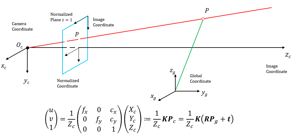
Fig. 2.1 Camera projection model with illustration of world coordinate, camera coordinate and image coordinate.

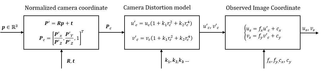
Fig. 2.2 Flow chart of projecting 3D points onto image coordinate where \(k_i\) is radial distortion paramter, \(f_x, f_y, c_x, c_y\) are camera instrinsic parameters, and \(r_c^2 = u_c^2 + v_c^2\).

In Fig. 2.2 the input point \(\mathbf{p}\) refers to the landmark in the world coordinate, the output \(u_s,v_s\) represents the corresponding observation.

Set the camera intrinsics \(\mathbf{K}\), then the relationship between pixel position and 3D space point is as follows:

\[\begin{split}\begin{equation} s_i \begin{bmatrix} u_i \\ v_i \\ 1 \end{bmatrix} = \mathbf{K}\text{exp}\left(\mathbf{\xi}^{\wedge}\right) \begin{bmatrix} X_i \\ Y_i \\ Z_i \\ 1 \end{bmatrix} \end{equation}\end{split}\]

To make it more compact, we write the projection model in matrix form:

(2.3)\[\begin{equation} s_i \mathbf{u}_i = \mathbf{K}\text{exp}\left(\mathbf{\xi}^{\wedge}\right)\mathbf{P}_i \end{equation}\]

2.2. Vision Processing Front End

For visual measurements, we track features between consecutive frames and detect new features in the latest frame.

For each new image, existing features are tracked using KLT sparse optical flow algorithm 1. Meanwhile, new corner featuers are detected 2 to maintain a minimum number (100 to 300) of features in each image. The detector enforces a uniform feature distribution by setting a minimum separation of pixels between two neighboring features.

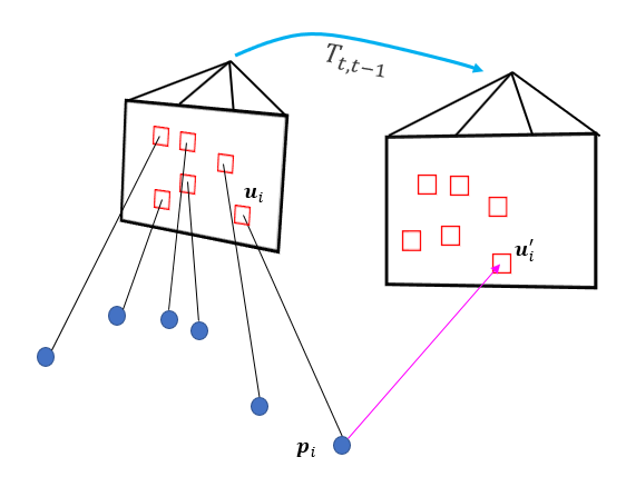
Fig. 2.3 Illustration of feature extraction and association for next step: triangulation.

2D features are first undistorted, then projected to normalized camera plane after passing the outlier rejection module, using RANSAC algorithm with a fundamental matrix estimation model, as shown in Fig. 2.3.

Keyframes are selected during this step. Two criteria are deployed during keyframe selection this procedure.

• The average parallax based on the previous keyframe.

  If the average parallax of the tracked features between the current frame and the latest keyframe is above a certain threshold, we treat this frame as a new keyframe.

  Not only translation but rotation as well can cause parallax.

• Tracking quality

  If the number of tracked features goes below a certain threshold, we treat this frame as a new keyframe. We need to adjust the strategy of feature extraction and avoid complete loss of feature tracks.

2.3. INSPVA Message Processing Front End

When Global Positioning System (GPS) is not available or reliable, VO applied on ground vehicles is an efficient tool for estimating the pose, which involves translation and rotation. However, VO inherently suffers from drifting issue due to constant iterations.

We add INSPVA data input as an auxiliary option to compensate inherent drift of VO on ground vehicles. One year ago, we published a paper called Heading Reference Assisted Pose Estimation for Ground Vehicles 5. In that paper, we introduced a framework to incorporate measurements from AHRS sensors into VO. We aim to build a agrph abstraction model, either a loosely-coupled model or a tightly-coupled model. In our proposed program, we modified the loosely-coupled model and built an INS error model as shown in Struct INSRTError.

Fig. 2.4 Illustration of INS + visual measurement model and graph formulation.

The loosely-coupled model is illustrated in Fig. 2.4. Let \(\mathbf{x} = \left[ x_0^{\mathrm{T}}, x_1^{\mathrm{T}}, \cdots, x_N^{\mathrm{T}} \right] ^{\mathrm{T}}\) be the state vector, where \(\mathbf{x}_0 \in \mathbb{R}^3\) denotes the orientation readings from INS sensor; Let \(\mathbf{z}_{ij}\) be the measurement vector. The ideal position measurement equation (ignoring noises) for VO and INS are:

(2.4)\[\begin{split}\begin{align} \mathbf{h}^{VO} (P_{k-1}^w, P_k^w) &= P_k^w - P_{k-1}^w \\ \mathbf{h}^{INS} (\phi_{k-1, k}) &= \sum_{i \in {\phi_{k-1, k}}} \mathbf{v}_i \cdot \Delta t_i \end{align}\end{split}\]

where \(\phi_{k-1, k}\) denotes all the INS messages in the interval of visual data from \(k-1\) th frame to \(k\) th frame; \(\mathbf{v}_i\) is linear speed reading and \(\Delta t_i\) is the time interval for this read.

The error functions are defined as:

(2.5)\[\begin{split}\begin{align} e_{trans} (\mathbf{P}_{k-1}^w, \mathbf{P}_k^w) & = \mathbf{h}^{VO} (\mathbf{P}_{k-1}^w, \mathbf{P}_k^w) - \mathbf{h}^{INS} (\phi_{k-1, k}) \\ e_{rot} (\mathbf{R}_k^w) & = {\mathbf{R}_k^w}^{-1} \mathbf{R}_{0k} \end{align}\end{split}\]

where \(\mathbf{R}_{0k}\) is the INS orientation reading at the \(k\) th frame.

2.4. (Optional) IMU Preintegration

The high frequency property of IMU (normally 100 ~ 200 Hz) and relatively large noise & bias makes it hard to integrate IMU data with visual data. To overcome this issue, IMU preintegration 3 is adapted and the handling of IMU biases as is included. So for the details of IMU noise and bias, preintegration and bias correction models, please read the paper. As the core task of SLAM does not include IMU sensor, we will only introduce it briefly.

1

B. D. Lucas and T. Kanade, “An iterative image registration technique with an application to stereo vision,” in Proc. Int. Joint Conf. Artif. Intell., Vancouver, Canada, Aug. 1981, pp. 24–28.

2

J. Shi and C. Tomasi, “Good features to track,” in Proc. IEEE Int. Conf. Pattern Recog., 1994, pp. 593–600.

3

C. Forster, L. Carlone, F. Dellaert, and D. Scaramuzza, “On-manifold preintegration for real-time visual–inertial odometry,” IEEE Trans. Robot., vol. 33, no. 1, pp. 1–21, Feb. 2017.

4

T. Barfoot, “State estimation for robotics: A matrix lie group approach,” Draft in preparation for publication by Cambridge University Press, Cambridge, 2016.

5

Wang, Han, Rui Jiang, Handuo Zhang, and Shuzhi Sam Ge. “Heading reference-assisted pose estimation for ground vehicles.” IEEE Transactions on Automation Science and Engineering 16, no. 1 (2018): 448-458.